NPF Analysis Tutorial
Introduction
Our aim here is to calculate the growth rate (GR) and formation rate (J) of particles in the size range 7-20 nm from aerosol number size distribution data.
This tutorial roughly follows: Kulmala, M. et al. Measurement of the nucleation of atmospheric aerosol particles. Nat. Protocols 7, 1651–1667 (2012).
Find representative diameters/times
Run the bokeh app
aerosol-analyzerfrom the terminalLoad the aerosol number size distribution data (
data.csv)Draw a region of interest (ROI) around the growing particle mode
Fit representative diameters/times using the mode fit method, maximum concentration method or the appearance time method.
Save the ROI as a JSON file (
npf_roi.json)
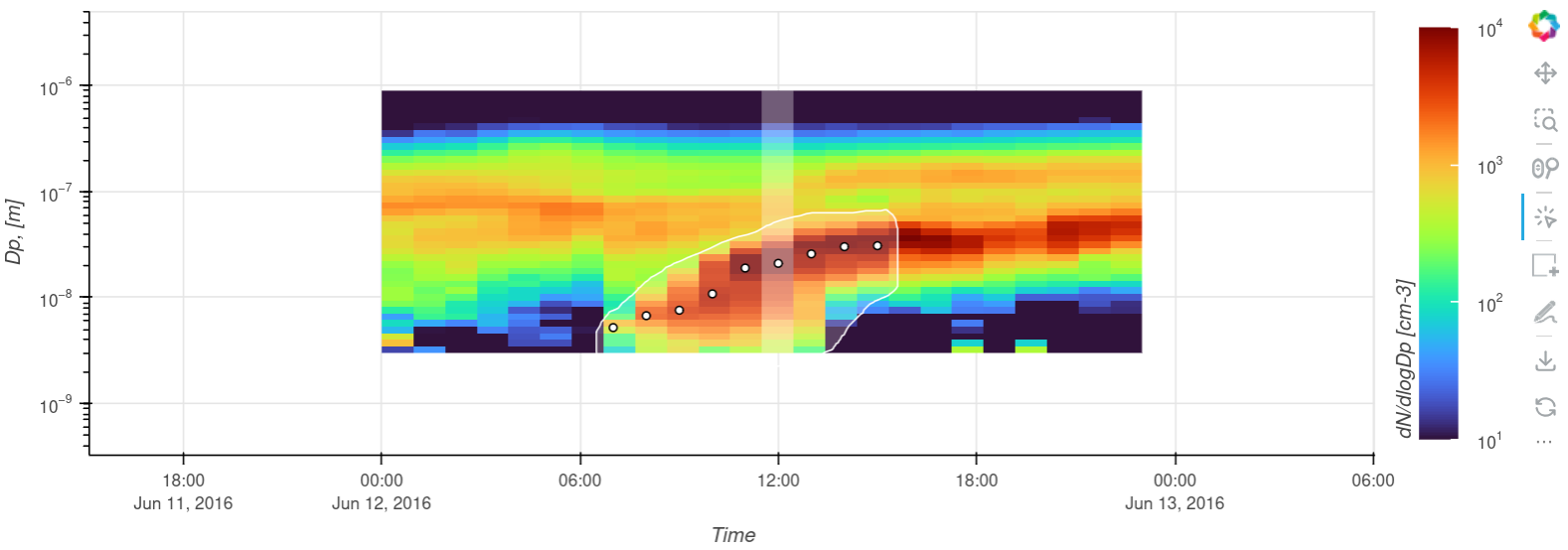 Figure 1: The number size distribution as a heat map with ROI drawn around the growing particle mode along with representative diameters/times found using mode fitting.
Calculate GR
Particle growth rate (GR) is defined as the rate of change of particle diameter
Next we write a script that does the following:
Load the JSON file with the ROI information
Extract the representative diameters/times and convert them to nanometers/hours.
Only select the representative diameters in the size range and fit a line through them
GR is calculated as the slope of the line fit in nm/h
import json
import pandas as pd
import numpy as np
import aerosol.functions as af

# Read a JSON file from disk
with open('npf_roi.json', 'r') as f:
    data = json.load(f)

# Extract the representative times/diameters from the ROI
time = []
diam = []
for i in range(len(data[0]["fit_mode_params"])):
    time.append(
        float(data[0]["fit_mode_params"][i]["time"])/(1000 * 60 * 60)) # hour
    diam.append(
        data[0]["fit_mode_params"][i]["diam"]*1e9) # nm

# Convert to numpy array
time = np.array(time)
diam = np.array(diam)

# Calculate the GR (done here between 7-20 nm)
idx1 = np.argwhere(((diam>7.) & (diam<20.))).flatten()
gr = np.polyfit(time[idx1],diam[idx1],1)[0] # nm/h

print(f'{gr:.2f} nm h-1')

# OUTPUT: 5.73 nm h-1
Calculate the formation rate (J)
The formation rate can be approximated by
The terms on the right-hand-side from left to right are the concentration term, the sink term and the growth term.
Calculating the sink term
# Load the number size distribution data
dndlogdp = pd.read_csv("data.csv",parse_dates=True,index_col=0)

# Convert from normalized concentrations to concentrations
dn = af.dndlogdp2dn(dndlogdp)

# Calculate the total sink term in the size range
diams = dndlogdp.columns.astype(float).values
idx2 = np.argwhere((diams>7e-9) & (diams<20e-9)).flatten()

sink_terms = []
for i in idx2:
    sink_term = (af.calc_coags(
        dndlogdp,
        diams[i]).values.flatten() *
    dn.iloc[:,i].values.flatten())
    sink_terms.append(sink_term)

total_sink = pd.DataFrame(
    index = dndlogdp.index,
    data = {0: np.sum(sink_terms, axis=0)})
Converting GR to dataframe
The GR is calculated only during the NPF event, otherwise it is assigned NaN.
# Convert the GR to Dataframe
gr_df = pd.DataFrame(
    index = pd.to_datetime(time[idx1], unit="h"), data = {0: gr})

# Reindex to the number size distribution data
gr_df = gr_df.reindex(dndlogdp.index)
Calculating the formation rate
# Calculate the formation rate
J = af.calc_formation_rate(
    dndlogdp,
    7e-9,
    20e-9,
    sink_term=total_sink,
    gr=gr_df)

# Calculate and print the mean formation rate
print(f'{np.mean(J["J"]):.2f} cm-3 s-1')

# OUTPUT: 0.48 cm-3 s-1